Executive Summary
Quantization is widely reported to be nearly free at 4 bits — on the evidence of aggregate benchmark scores. This paper asks whether that average conceals capability-specific damage, using two capabilities — long-context retrieval and multi-step arithmetic — measured on the same model, the same component set, and the same paired per-item design.
Headline Discoveries:
- 4-Bit Quantization is “Nearly Free”: Compressing weights to 4-bit (NF4 or
int_group) causes no statistically detectable damage to either long-context retrieval or multi-step arithmetic onQwen2.5-1.5B-Instruct. NF4 gives retrieval dz = +0.221 (1.01× the measured noise band) and arithmetic dz = −0.079 at n=96;int_groupat 4 bits gives +0.205 and +0.164 at n=48. The consensus is confirmed, not refuted. - 3-Bit Quantization Breaks Models Asymmetrically: At 3-bit (
int_group— the only quantizer that reaches 3 bits, since NF4 has no 3-bit form), both capabilities fail, but Retrieval suffers 3.2× the standardized damage (dz = +1.876) compared to Arithmetic (dz = +0.589). Damage depends on precision and differs by capability! And this asymmetry needs no component map, no multiplicity correction and no significance gate — it falls out of whole-model interventions on identical items. - Quantization Can Help Performance: Out of 26 retrieval-sensitive components, 8 components actually IMPROVE retrieval NLL when quantized to 3-bit! The largest effect is
mlp_block__L27(dz = −1.468). They do not cluster — not by depth (Mann–Whitney p = 0.96), not by module type (Fisher p = 1.00) — and across all 56 components the layer index carries no information about the direction of the effect (Spearman ρ = −0.051). - Standard Ranking Methods Are Flawed: Traditional methods rank layer sensitivity without significance tests or power analyses. Localizing the damage to components is much harder than it looks, and most of this paper is about why:
- The significance gate does not travel: defined as an absolute threshold on a raw metric — the standard noise-floor construction, and the one this study pre-registered itself — it cannot compare two capabilities against the same bar, it structurally excluded one of the two capabilities from ever registering an effect, and it reverses its verdict on a replication of an effect that reproduces at p = 0.0001 (§4.1).
- Component power models fail empirically: the natural model for extrapolating component effect sizes is wrong by an order of magnitude, conservatively, and it is falsified twice, from independent directions (§4.2).
- Absolute values manufacture fake agreement: a documented, defensible-sounding decision in the primary test consumed the wrong quantity, and the paper exhibits the eight measured components that would have inverted its reading (§4.3).
- Selected extrema regress: every effect size selected as an extremum shrank on re-measurement — three for three, by 20–45%, once far enough to cross a pre-registered decision threshold (the Winner's Curse, §4.4).
The resulting 3-bit component map is reported with its coverage stated: adequately powered for 21 of 56 components (37%). The primary pre-registered test of whether the two capability maps differ is inconclusive, and is reported as such.
1Introduction: Beyond Global Perplexity Averages
The Problem: Does “4-Bit Is Free” Hide Hidden Destruction?
Quantization — post-training compression of model weights from FP32/FP16 down onto a coarse N-bit grid — is reported to be nearly free. Aggregate benchmark scores barely move at 4 bits, and that finding underwrites a great deal of deployment practice. But an aggregate is an average, and an average can hide the destruction of a specific capability while the mean stays flat.
The concern is not hypothetical in the method itself. Existing approaches to allocating precision decide what to protect by asking which weights most damage perplexity — a single, global average over all tokens. If different capabilities depend on different parts of a model, then optimizing a global average is the wrong objective, and a method that protects the weights perplexity cares about may be protecting the wrong ones for any particular deployment.
So the question is: do different capabilities depend on different parts of the model, and if so, can precision be allocated by capability rather than uniformly? Both answers are results:
- If the capability maps differ — a model can be compressed differently depending on what it is deployed for.
- If the maps coincide — there is a shared critical set of layers, which is a stronger and more surprising claim about how models are organized.
This is also why testing one capability alone is not a result. “Some layers matter more than others” is true of any capability measured in isolation; you will always find a ranking. It is the contrast between two capabilities that carries the information — which is why both are measured here from the first run, on the same items and the same component set, rather than one being bolted on later.
The Findings at a Glance
- The Premise Needs Correction at 4 Bits: At 4-bit NF4 on this model, neither capability moves detectably — retrieval sits at 1.01× the measured noise band, arithmetic does not move at all. The “4-bit is free” consensus is confirmed, not refuted.
- Asymmetry Emerges at 3 Bits: The damage is real, but it is real at 3 bits, where both capabilities break and retrieval takes 3.2× the standardized damage of arithmetic. Quantization damage is precision-dependent and capability-asymmetric — and the asymmetry is measurable in aggregate before any component map is drawn.
- Localizing Layer Damage Is Extremely Hard: Component-sensitivity work in quantization computes a score and ranks it. Across every method surveyed, none reports a significance test, a noise floor, a multiplicity correction, a power analysis, or a replication. Importing that machinery — as a study comparing two capabilities must — surfaces three things a ranking cannot:
- the natural significance gate is non-comparable across capabilities and unstable under replication;
- there is no model for the statistical power of a component ablation, and both obvious candidates fail by measurement;
- selected effect sizes shrink on re-measurement — once far enough to cross a threshold that had been fixed in advance.
None of that statistical machinery is novel. Significance testing, power analysis and selection correction are standard in neuroimaging, genetics and econometrics; this paper cites those literatures rather than re-deriving them. The finding is their absence here — and what that absence costs once the question is a comparison rather than a ranking.
The 3-bit component map is therefore reported with its coverage stated — adequately powered for 21 of 56 components — and the pre-registered test of whether the two capability maps differ comes back inconclusive. It is reported as inconclusive, with a whole section given over to the claims that are not being made.
2Experimental Setup & Pre-Registration Standards
Every decision rule in this study was fixed in writing before any number was produced, and the choices are enforced by automated guards in code rather than by discipline.
Model & Tasks
- Base Model:
Qwen2.5-1.5B-Instruct, float32, on a single GPU. - Capability 1 (Long-Context Retrieval): needle-in-a-haystack at 4k tokens, scored by exact string match on inserted passcodes.
- Capability 2 (Multi-Step Arithmetic): GSM8K math word problems, scored on the final number.
- Both tasks are boolean and grader-free — no model-as-judge anywhere in the loop — and both are measured from the first run rather than added later, for the reason §1 gives.
Quantization Methodology
- Simulated grid quantization: weights are rounded onto the grid an N-bit quantizer would produce and stored in the original dtype (the grouped-integer quantizer
int_groupuses group size 64). This is standard practice, and it is the only way to intervene on a single attention head — production export libraries cannot do it. - Exact NF4 validation: the NF4 implementation reproduces
bitsandbyteselement for element, with zero differing elements — on Gaussians, on real weights, and on non-contiguous column views. - Two independent intervention paths: weight mutation and runtime materialization are asserted to produce bitwise-identical logits on the real device before every run.
- Grouped-Query Attention (GQA) precision: with
n_kv < n_q, “quantize head h” has two non-equivalent definitions, and the wrong one is arithmetically well-formed and silently wrong. Both are implemented as distinct component types with disjointness asserted within each, and the mapping suite is mutation-tested: anh // n_kvgroup-map typo, ano_projrow/column swap, and a one-head offset fail 8, 5 and 2 tests respectively.
Dual Evaluation Metrics
- Search metric (continuous): teacher-forced Negative Log-Likelihood (NLL) over the answer span — deterministic, continuous, one forward pass — measured paired per item (Δi = NLLi(quantized) − NLLi(baseline)). Item-to-item difficulty is large, and pairing cancels it.
- Confirmation metric (discrete): boolean exact match, tested with McNemar on discordant pairs.
Both are recorded on every run, so the relationship between them is measurable rather than assumed.
Difficulty Calibration
A saturated eval has no headroom. If the unmodified model scores ~100%, no single-component intervention can produce a measurable effect — and the study would dutifully return “no effect” after building an instrument with no dynamic range. So difficulty is calibrated before any sweep, and the choice is enforced in code:
- A ladder of needle variants is evaluated, and the hardest one is selected whose unmodified accuracy lies in a pre-registered band, whose uniform-quantization drop is significant by McNemar, and whose NLL increase clears the measured noise floor.
- The chosen variant is then frozen for every later rung.
- The runner reads the calibration record and refuses to start if a config names a different variant — or a different model, context length, device or dtype.
Why enforce it in code rather than in prose? Because an earlier version of this project carried the requirement as a comment — and the comment was violated by the config directly beneath it.
The Pre-Registration, and One Amendment
Decision rules were fixed in writing before any number was produced. Every subsequent change is recorded in an amendment log with its date, its reason, and an explicit check of whether it alters any prior verdict.
One amendment concerns the calibration above directly. The headroom band's upper bound was pre-registered at 0.98. Measuring a second model, the frozen variant scored 47/48 = 0.97917 and passed — inside the band by 0.0008, in a setting where one item at n=48 is worth 0.0208. The rule was discriminating at a resolution 26× finer than the measurement can represent, and one more correct item would have failed it. So:
- The ceiling was moved to 0.96.
- The change was verified against all 36 baselines in the project: exactly one verdict changes — the run that exposed the problem.
- A more principled fix — expressing headroom in items rather than in a fraction — was rejected, because it would have invalidated the n=12 screen that selected the very variant this project is built on. That rejected rule is written down, unadopted, with its counterfactual.
3Headline Result: Precision-Dependent & Capability-Asymmetric Damage
The experiment is deliberately blunt. I quantize every linear weight in Qwen2.5-1.5B-Instruct to 2, 3 and 4 bits with a group-wise integer quantizer (int_group, group size 64), then measure two capabilities on identical items:
- Long-context retrieval — needle-in-a-haystack at 4k tokens, scored by exact string match on the inserted passcode. Baseline accuracy 0.896 (n=48).
- Multi-step arithmetic — GSM8K word problems, scored by exact match on the final number. Baseline accuracy 0.750 (n=48).
How the Effect Is Measured
- Paired per item. Each item's damage is its own difference in negative log-likelihood (NLL — how surprised the model is by the correct answer): Δi = NLLi(quantized) − NLLi(baseline).
- Aggregated with a sign-flip permutation test.
- Bit-identical baselines across the three separate processes that produced them — so the three rungs of the ladder differ in nothing but precision.
All figures below are int_group (group size 64) at the stated width, n=48 per capability.
Weight Precision (int_group, group size 64)
  2-bit  │ Retrieval: Broken (acc 0.000, dz +9.061)  │ Math: Broken (acc 0.062, dz +6.759)
  3-bit  │ Retrieval: BROKEN (acc 0.167, dz +1.876)  │ Math: BROKEN (acc 0.438, dz +0.589)  <-- 3.2x ASYMMETRY
  4-bit  │ Retrieval: Intact (acc 0.771, dz +0.205)  │ Math: Intact (acc 0.646, dz +0.164)  <-- NEARLY FREE
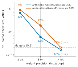
int_group, n=48 per rung. Both capabilities are intact at 4 bits and broken at 3; at 3 bits retrieval takes 3.2× the standardized damage of arithmetic. Open markers are McNemar non-significant at α=0.05. This is the paper's headline result, and it uses none of §4's machinery.Key Quantitative Comparison Table
Capability & Quantizer (int_group) |
4-Bit Precision | 3-Bit Precision | 2-Bit Precision |
|---|---|---|---|
| Retrieval (dz effect size) | +0.205 (n.s.) | +1.876 | +9.061 |
| Retrieval accuracy (n=48) | 0.896 → 0.771 | 0.896 → 0.167 | 0.896 → 0.000 |
| Arithmetic (dz effect size) | +0.164 (n.s.) | +0.589 | +6.759 |
| Arithmetic accuracy (n=48) | 0.750 → 0.646 | 0.750 → 0.438 | 0.750 → 0.062 |
What is dz?
Cohen's dz is the standardized paired effect size — how big the per-item damage is relative to how much it varies from item to item:
A threshold of |dz| ≥ 0.2 is the practical-significance cutoff used throughout this paper.
Why 3-Bit Reveals What 4-Bit Conceals
At 4 bits neither capability moves detectably — and I say precisely which hurdle each one fails.
- Retrieval: dz = +0.205, which is fractionally above the 0.2 practical-significance threshold, not below it. It fails on significance instead: permutation p = 0.158, McNemar p = 0.109.
- Arithmetic: fails both hurdles — dz = +0.164 is below the effect-size threshold, and permutation p = 0.308, McNemar p = 0.267.
So the "4-bit is nearly free" consensus is confirmed, not refuted — and I report it as a confirmation precisely because the framing that motivated this work predicted the opposite.
At 3 bits both capabilities break — but they break unequally. Retrieval takes 3.2× the standardized damage of arithmetic (dz +1.876 against +0.589). Integer bit widths are too coarse to separate the two by break point — both are intact at 4 and broken at 3 — but at the one width where both move, the magnitude separates them decisively.
Here is the part worth pausing on: this result needs none of the rest of the paper. No component map. No multiplicity correction. No significance gate. No importance vectors. It is four whole-model interventions on two capabilities, measured on the same items. Every methodological finding in §4 leaves it standing.
The Quantizer Caveat: Anchoring, Not Assuming
The quantizer on the ladder is not the one people deploy. nf4 — the format the 4-bit literature actually uses — has no 3-bit form, so the ladder has to run on a parameterizable integer quantizer. At 4 bits, where both formats exist, I compare them paired on identical items against a bit-identical baseline:
- Retrieval: difference −0.0064 (p = 0.816, n=48).
- Arithmetic: difference +0.0090 (p = 0.729, n=24).
- Whole-model NF4 at n=96 gives retrieval dz +0.221 and arithmetic −0.079, against
int_group@4's +0.205 and +0.164 at n=48. The arithmetic pair differs in sign, and neither estimate is distinguishable from zero — that is the entire content of the comparison.
These are failed rejections, NOT equivalence claims (§7). I do not claim the two formats are interchangeable — only that I cannot distinguish them at the one width where the comparison is even possible.
Does Component Importance Transfer Across Precision? A Preliminary Result
The map in §5 is drawn at 3 bits; deployment happens at 4. So the first question a practitioner asks is whether the ordering survives a precision change. I report the only direct measurement I have — with its limits attached, not appended afterward. Re-measuring six components at 4-bit NF4 on the same 96 items:
- Two of the six reverse sign.
- The sharpest case is the worst one:
attn_block__L12carries the strongest dz in the entire 3-bit top group (+1.349) and moves the other way at 4 bits (dz −0.477). A 3-bit map used to decide what to protect in a 4-bit deployment would rank that component near the top and be wrong about its direction. - The limits are severe: n = 6 components, Spearman ρ = +0.600 — positive, consistent with partial transfer, and not significant (six points need ρ ≈ 0.83 at p < 0.05). Both reversals sit between values that are near-null at both precisions.
I put it here rather than in the limitations because it is preliminary evidence on a question this literature has no evidence on at all, and burying it invites it to be read as a caveat I am conceding rather than a measurement I made. It is explicitly NOT the pre-registered rank-transfer test, which was a 5-vs-5 group contrast and was formally withdrawn on its own cost criterion (§8).
A Bit Width Is Not a Fixed Amount of Damage Across Model Scales
Repeating the 3-bit intervention on Qwen2.5-3B — on byte-identical items, the two models sharing a tokenizer — destroys both capabilities outright:
- Retrieval: 0.979 → 0.000 (n=48).
- Arithmetic: 0.896 → 0.042 (n=48).
That places the 3B at 3 bits inside the 1.5B's two-bit regime. The precision at which a capability breaks is itself model-dependent. The direct consequence: I report NO cross-model asymmetry ratio, because comparing the two models at a shared bit width compares a break point against a floor. It also raises a question about designs that compare sensitivity across model scales at a fixed format — but that is one measurement on one pair of models, so it is a question, not a refutation.
4Four Methodological Pitfalls in Layer-Sensitivity Research
Most quantization work ranks components without ever testing whether the ranking means anything. Import statistical machinery into that setting and four defects fall out immediately. Be clear about what they are: none of the four is a statistical discovery, and I do not claim any of them as one. All four were found with machinery this field simply does not use — and that absence is the finding.
One further guard is worth naming up front. §4.5 measures what a single piece of that machinery was actually worth: a guard added for one purpose caught an unrelated error two days later, in a part of the pipeline no test covered. I say so here so the four findings below read as measured rather than urged.
Pitfall 1: Absolute Raw Metric Gates Fail & Reverse on Replication
Localizing damage means deciding which per-component effects count at all. That decision needs a gate — and the obvious gate breaks in two separate ways.
- The Common Approach: define a "noise floor" from the baseline itself. Bootstrap the baseline mean over ≥20 items per capability, then take half the width of its 95% confidence interval as a noise band. An effect landing inside the band is not a finding. This is what I pre-registered (§2), because it is what the brief specified.
- Why It Fails: the band is an absolute threshold on the raw metric, derived per capability from that capability's own baseline variability. So the two capabilities are not being asked the same question — they face different bars entirely:
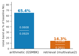
| (n=96) | baseline NLL | band | band as % of baseline | largest component effect | band ÷ effect |
|---|---|---|---|---|---|
| retrieval | 0.2011 | 0.0288 | 14.3% | +0.0641 (mlp_block__L13) |
0.45 |
| arithmetic | 0.0929 | 0.0608 | 65.4% | +0.0091 (attn_block__L22) |
6.69 |
Arithmetic had to move its NLL by 65% of its own baseline value to register anything. Retrieval had to move 14%. That is a 4.6× difference in relative stringency that nothing in the research question asks for — and it follows mechanically from the construction: a capability whose baseline mean is less precisely known gets a larger band, hence a harsher absolute bar. But "how precisely do I know the baseline mean" is not the same question as "how large must an effect be to matter."
- Result: this is not a matter of degree. Simulated against the measured per-item spreads, the arithmetic gate has power 0.00 at every n up to 1536, at every effect fraction — its band sits 6.7× above the largest effect that is actually present. One capability was gated; the other was structurally excluded from ever registering anything, in a study whose entire object is comparing the two.
- Replication Flaw: the same gate flips its verdict on a clean replication.
mlp_block__L27improves retrieval NLL by −0.0330 (dz = −1.468) at seed 2024. Re-measured on a disjoint item set at seed 2025 — zero shared item ids — it returns −0.0295 (dz = −1.194) at p = 0.0001. The effect replicates. The verdict does not!
| item draw | ΔNLL | band | band gate | dz gate |
|---|---|---|---|---|
| seed 2024, n=96 | −0.0330 | 0.0288 | PASS | PASS |
| seed 2025, n=48 | −0.0295 | 0.0429 | FAIL | PASS |
Nothing changed except which documents were drawn. That draw produced a wider baseline CI, the band moved up above the effect, and PASS became FAIL. A threshold derived from the baseline sample is a property of the sample, not of the effect it is supposed to gate.
- The Solution: a fixed, standardized effect-size threshold, |dz| ≥ 0.2. I replaced the gate before drawing any map — adopted 13 minutes before the first map was computed, with no ranking and no significance verdict produced under either gate beforehand. And both verdicts are reported for every component throughout, so the amendment's effect is visible rather than asserted.
Again, to be exact about the claim: neither of these two findings is a statistical discovery, and I do not present them as one. That an absolute threshold is non-comparable across conditions, and that a sample-derived one is unstable, is textbook. What is notable is that this literature has never had to notice — §9 documents the absence across every method I surveyed. When testing is imported into a field that only ranks, the very first gate you would reach for turns out to be non-comparable across tasks, unstable under replication, and to leave most of the resulting map inadequately powered.
Pitfall 2: Component Power Models Fail Empirical Tests
How many items does a component sweep actually need? Answering that requires a model of how a single component's effect — and its item-to-item spread — relate to the whole-model intervention. No such model exists in this literature, because this literature does not do power analysis. So what follows is not offered as a correction to standard practice; the absence is the finding.
Two candidate models are the obvious ones to try. Both fail.
- Multiplicative scaling — degenerate, for a structural reason:
di(f) = f · diThe sign-flip statistic is scale-invariant, so this model reports a component carrying 1% of the effect as exactly as detectable as the whole model. That is not an approximation error you can bound and live with — the model cannot express the question.
- Additive scaling — shrinks the signal but keeps the residual:
di(f) = f · mean(d) + (di − mean(d))This implies that item-to-item spread is invariant to the size of the intervention. It is not.
I falsify the additive model from two independent directions.
- Across 56 components at one precision: the median component's spread is 0.101× the whole model's — 0.0360 against the whole-model arm's 0.3577.
- Across the same components at two precisions: spread scales by 0.357× going from 4 bits to 3 bits.
Spread shrinks with component granularity and with precision. Crucially, the error runs one way: it is conservative. Overstating spread understates dz, which understates power — so every "I lack power" conclusion drawn from such a grid is too pessimistic.
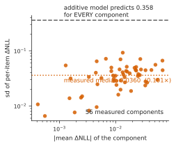
What this leaves. A third model must let spread shrink with intervention size, and the two measured ratios (0.101× and 0.357×) are its constraints. There are 62 measured single-component effects available to fit and cross-validate one — the 56 components of the 3-bit sweep, plus six re-measured at 4 bits for the transfer pilot. I name the requirement and supply the constraints. I do not fit the model.
Pitfall 3: Using Absolute Values (abs(mean_delta)) Manufactures Fake Agreement
The hardest defect to find is not a typo. It is a documented decision that is defensible in general and wrong for the one claim it feeds. My primary test correlates two capability importance vectors, and both were built from abs(mean_delta) — under an explicit comment saying why.
- The Common Logic: the comment in the code read, “Sign is not meaningful for ranking: a component whose quantization HELPS is still an influential one.” That sentence is true of influence.
- Why It Fails: it is wrong for a test asking whether two capabilities are damaged in the same places. Under absolute values, a component that helps one capability and hurts the other pushes the two maps toward looking identical — manufacturing agreement out of opposite behavior.
- How It Was Caught: before either script ran, on the argument alone. The measured instances arrived afterwards.
- Impact: there are eight of them. Every component whose quantization improves retrieval while damaging arithmetic would have been counted as agreement (§6).
- What I Do Not Claim: no verdict changed because of this (§7). I report the defect, not a reversal.
- The Audit: an audit for the same shape of mistake found two more — one in the boolean path, one in a silent default.
Pitfall 4: Winner’s Curse (Selection Bias) Inflates Top Component Effects
The Mechanism: scan a pile of noisy measurements, pick the largest, report its magnitude — and you have over-estimated it. This is not a new phenomenon and I do not claim it as one. Neuroimaging peak inference states it directly, and the canonical treatment is Inference on Winners (Andrews, Kitagawa & McCloskey, QJE 2024). The structural match is exact: that literature handles the correlated-maximum case, which is precisely mine at 56 correlated components. The accepted correction is data-splitting, and my fresh-item re-measurements are that procedure, with zero shared items.
| What was selected | Selected | Data-split | Shrinkage |
|---|---|---|---|
| the calibrated variant, chosen partly because its effect looked large | dz 0.395 | 0.221 | −44% |
| the largest arithmetic component at n=96 | dz +0.150 | +0.082 | −45% |
| the only arithmetic component to clear the gate | dz +0.246 | +0.197 | −20% |
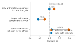
I contribute the instances, not the phenomenon. The third row is the one that matters: it crossed a pre-registered threshold, DETECTED → NOT DETECTED, on 0.003 in dz. And the surrounding literature selects extrema, reports their magnitudes, and applies neither correction nor re-measurement.
Selection breaks the interval, not only the estimate. This is the sharper point in Inference on Winners:
- Selection leaves roughly a 90% chance of over-estimating the effect.
- Conventional confidence intervals on selected quantities have true coverage below 82% at a nominal 95%.
- So I classified every interval this paper reports by whether its quantity was selected on the same data the interval is computed from. One of five is affected (full audit in Appendix A).
- The affected one:
mlp_block__L27’s arithmetic dz interval [+0.176, +0.319] is computed on the very data that selected it — the only component of 56 to clear the gate — and is therefore post-selection. - The replacement: [+0.119, +0.274], computed on disjoint items for what is by then a pre-specified component, and therefore valid. I report this second interval as the effect’s interval, and present the first only as the selected estimate that prompted the re-measurement.
- A caveat on the 82% figure: both of mine are bootstrap 90% intervals, so the quoted 95% coverage number bounds the degradation rather than describing it.
Theory and measurement corroborate — independently. The two results were obtained without reference to each other, and they agree.
- Theory says selection makes the interval both too narrow and centered too high, so correcting shifts the plausible range downward, toward and below the 0.2 margin.
- Measurement on disjoint items landed at dz = 0.197 — below it.
- Neither was derived from the other: the QJE result predicts a direction without ever seeing my data, and the fresh-item run measures a value without invoking the theory. Two routes, one theoretical and one empirical, reaching the same conclusion is stronger than either alone — and materially stronger than the framing they replace, which was merely that the selected interval straddled the margin.
Why Holm does not substitute for this. Multiplicity correction does not correct effect estimates. The two adjustments pull on different quantities in different directions: winner’s-curse adjustment shrinks Z-scores toward zero, while multiplicity adjustment shrinks p-values toward one. My Holm correction was never going to fix the estimates — which is exactly why the re-measurements were necessary rather than redundant.
What One Guard Was Actually Worth
This paper argues that experiments of this kind need machinery — assertions, provenance, pre-registration — that the surrounding literature does not use. That argument is easy to make and hard to evidence, because a guard that works produces nothing to point at. Here is one that produced something.
The guard. It was a storage-layout change, and nothing more:
- The Original Layout: noise floors were stored one file per (model, capability, variant, context length), with the run that measured them recorded inside the file.
- The Collision: two runs sharing those four attributes therefore wrote to the same path, and a later run silently replaced an earlier one’s floor.
- What Did Not Break: the loading code required the run to match and raised — so nothing was ever gated by the wrong band. But the earlier run’s floor was gone.
- The Change: I moved floors to
noise_floor/<run>/<key>.json, putting the run in the path, so the collision cannot occur. That change was made for that reason and no other.
Two days later, an unrelated defect. The figure carrying §4.1 — the noise band as a percentage of baseline NLL (negative log-likelihood) — took its numerator from one run’s summary and its denominator from a different run’s, at a different n on a different item set. It plotted 51.9% / 14.7% where the correct values are 65.4% / 14.3%.
Why nothing caught it is what makes this defect class dangerous: the bars looked plausible and still supported the claim. A 51.9-versus-14.7 asymmetry argues §4.1 correctly while misstating its central number by 13.5 points. No assertion fired because none existed — the script read two files and divided.
The fix requires the guard. The corrected figure asserts that both terms come from the same run, by reading the run field of the floor it loaded and comparing it to the run requested. Under the original flat layout that assertion could not have been written: the file’s location carried no run, and its contents were exactly what the mix-up had already bypassed. A change made to prevent silent overwriting turned out to be what made an unrelated class of error checkable at all.
I report this because it is the honest form of the argument. “Provenance guards are worth their cost” is not a claim I can support by having had no failures. What I can show is a guard added for one purpose catching a different error two days later, in a part of the pipeline — figure generation — that no test covered at all. I have since added tests asserting each figure’s plotted values against their source files. And the admission that goes with it: the first version of those tests re-derived the numbers independently and PASSED with the defect deliberately reintroduced. That is the same failure one level up — which is why they now assert on what the plotting code returns.
5The 3-Bit Component Map & Coverage Analysis
With the gate replaced, I swept all 56 components — 28 attention blocks and 28 MLP blocks, one per layer — at 3-bit precision, n=96, on both capabilities. Each component is quantized alone against a shared baseline (retrieval accuracy 0.917 at n=96, arithmetic 0.729 at n=96), paired per item, and corrected across the whole sweep with Holm–Bonferroni.
Retrieval Localizes — 26 of 56 Components Clear the Gate
The structure is real, and it is not confined to one region of the network:
- Early attention:
attn_block__L0, dz +0.958. - Mid-depth attention:
attn_block__L12, dz +1.349 — the largest damaging component in the map. - MLP blocks throughout the depth, early to late.
Of those 26, 18 are damage and 8 are improvement — components whose quantization lowers retrieval NLL. §6 treats that class, which is considerably larger than the single anomaly it is easy to mistake it for.
The Two Gates Disagree on 16 of 56 — and Every Disagreement Runs the Same Way
The original band gate admits 10 components. The standardized dz gate admits 26. And no component is admitted by the band and rejected by dz — the disagreements are one-directional, all 16 of them.
So the replacement is strictly more permissive on this data. I state that plainly because it is the opposite of what a reader may expect from a rule adopted to fix a broken gate — and because it was predicted in writing, with the affected components named, before the map was computed.
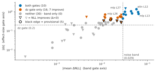
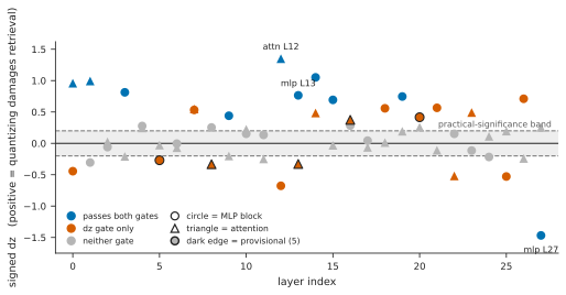
power_measured.py, which assumes no effect-scaling model). Positive dz means quantizing the component damages retrieval; the eight negative gated points are the improving class of §6.Coverage Is Part of the Result, Not a Caveat
How much of the map can I actually see? I answer by resampling each component's own measured per-item deltas — the plug-in bootstrap, with no effect-scaling model in it (§4.2):
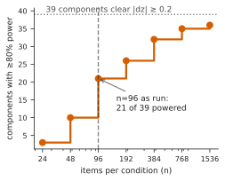
- 21 of 56 components (37%) are adequately powered at n=96.
- Of the 39 components whose effect clears the practical threshold, 18 are underpowered.
- Of the 26 I report as significant, five are provisional — detected below 80% power, named individually in the results, and marked with dark edges in the component map.
- On the measured ladder: n=192 would cover 26 of the 39, n=384 would cover 32, and n=768 would cover 35.
Which forces one reading rule on anyone using this map: an absent bar is not evidence of an absent effect (§7).
Arithmetic Resolves Almost Nothing — and Its One Detection Evaporates
At n=96, no arithmetic component clears the gate on either metric. Equivalence testing per component against the pre-registered margin returns:
- n=96: 0 detected, 7 equivalent to zero, 49 indeterminate — the data excludes neither a real effect nor none.
- n=384 (I quadrupled the arm): 1 detected, 48 equivalent, 7 indeterminate.
The single detection is mlp_block__L27 at dz +0.246 [+0.176, +0.319] — and I report its data-split value in the same breath, because it is the one number a reader would otherwise carry forward wrongly. That component was selected as the largest of 56, so its estimate is subject to the winner's curse (§4.4). Re-measured on disjoint items at the same n, it returns dz +0.197 [+0.119, +0.274] — below the 0.2 margin.
So the detection is not one I carry. The honest count for arithmetic at n=384 is zero components detected on unbiased re-measurement, with 48 of 56 equivalent to zero within a standardized margin of 0.2. The equivalence result is the reportable one; the detection is an instance of §4.4's phenomenon, not a finding about the model.
What I Do Not Write: That Arithmetic Fails to Localize
This is the caveat that matters most in §5. Against the largest effect actually present, the adopted gate has only 0.225 power at n=96 — measured by resampling that component's own per-item deltas, not extrapolated through the effect-scaling model §4.2 falsifies. A pre-registered null is uninterpretable unless the gate's power against a stated alternative is known, so the reportable statement names it (§7).
The Primary Test Is Inconclusive
The study's headline question — do the two capability maps differ? — is decided by a Spearman correlation between the two signed importance vectors over the shared component set. The answer is a shrug:
- ρ = −0.0014, against a permutation null of mean −0.0016 and sd 0.1365.
- p ≈ 0.50 in both directions, with top-10 overlap 2.
- Neither pre-registered condition is met. Maps differ requires ρ significantly below the null. Maps coincide additionally requires both capabilities to localize — and arithmetic does not.
I report it as inconclusive and construct no third narrative. What ρ ≈ 0 does and does not license is stated in §7, where the boundary on every claim in this paper is drawn in one place.
6The Surprising “Helping” Class: Quantization Improves Retrieval
Eight of the 26 components that clear the gate improve retrieval NLL rather than damaging it! Quantizing them to 3-bit lowers the negative log-likelihood the model assigns to the correct answer span. That is an NLL claim, not an accuracy claim — the boundary is drawn at the end of this section.
This is a class, not an anomaly — and I state its size before examining its largest member, deliberately, because the reverse order invites the reading that one odd component was found and the rest of the map is well-behaved. Eighteen components damage retrieval; eight improve it.
The Top 8 Retrieval-Improving Components
| component | ΔNLL | dz | 95% CI | power |
|---|---|---|---|---|
mlp_block__L27 | −0.0330 | −1.468 | [−0.0375, −0.0286] | adequate |
mlp_block__L12 | −0.0265 | −0.677 | [−0.0345, −0.0191] | adequate |
mlp_block__L5 | −0.0265 | −0.270 | [−0.0481, −0.0102] | provisional |
attn_block__L13 | −0.0214 | −0.329 | [−0.0358, −0.0103] | provisional |
mlp_block__L0 | −0.0156 | −0.444 | [−0.0228, −0.0089] | adequate |
attn_block__L22 | −0.0113 | −0.519 | [−0.0156, −0.0069] | adequate |
attn_block__L8 | −0.0109 | −0.332 | [−0.0177, −0.0047] | provisional |
mlp_block__L25 | −0.0045 | −0.529 | [−0.0062, −0.0028] | adequate |
mlp_block__L27 is the largest of eight, not the only one — 1.2× the next by raw effect and 2.8× the next by dz. It is also the largest |dz| in the entire map in either direction, exceeding even the largest damaging component (attn_block__L12, +1.349). It is an extreme case of a class — a stronger claim than a singular anomaly, and a weaker one than a mechanism.
Two bounds on the class, stated up front. Three of the eight are provisional (below 80% power at n=96) and are marked as such throughout — but the class survives their removal at five, including both endpoints. And the remaining 14 components with negative point estimates do not clear the gate, so I make no claim about them. Whether the class is eight or larger is a question of n, not of sign.
Properties of the Helping Class
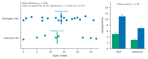
- No spatial clustering. The eight sit at layers 0, 5, 8, 12, 13, 22, 25 and 27 — spanning the model end to end — with a median of 12.5 against the damaging set's 14.0 (Mann–Whitney p = 0.96). Across all 56 components, layer index carries no information about the direction of the effect (Spearman ρ = −0.051, p = 0.71). I report this negative result because the obvious reading of a single late-MLP anomaly — “the last block is special” — is not what the class supports:
mlp_block__L0is at the opposite end of the network and improves too. - No module-type preference. The eight split 5 MLP / 3 attention against 11 / 7 among the damaging components — indistinguishable (Fisher exact p = 1.00). Helping is not a property of a region or of a module type in this map.
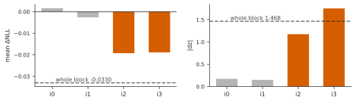
- Sub-block granularity — concentrated, but “concentrated” is not “two of four chunks are zero.” Decomposing
mlp_block__L27into four chunks of its intermediate dimension, against 25% each under an even split:- Two chunks carry 58.3% and 57.2% of the block effect.
- The other two are not nothing: one carries 8.0% in the same direction, and one carries −4.9% — the opposite sign, a small damaging contribution (dz +0.173) inside a block whose net effect is a large improvement. I state both rather than rounding them to zero: a chunk running the other way is evidence against the strongest version of the concentration claim.
- The four chunks sum to 118.6% of the block effect. Quantization is not linear and each chunk is quantized independently, so exact additivity was never expected.
- Monotone in perturbation strength. At 4 bits the same component gives −0.0068 (dz −0.780); at 3 bits, −0.0330 (dz −1.468). Stronger perturbation, larger improvement — which is what “this block's contribution is net-harmful for this objective” predicts, and the opposite of “mild-perturbation regularization,” which predicts a peak at intermediate strength. But two points is not a curve, and 2 bits cannot extend it: the model is destroyed there, so a component measurement says nothing.
- Refuted mechanism. I proposed distributional flattening via the tied output head, which predicts that items the baseline answers correctly should get worse while incorrect ones improve. Split by baseline correctness, both subsets improve by the same amount (−0.0339 on 43 correct items at p = 0.0001; −0.0311 on 5 incorrect). The account is refuted, and no mechanism has replaced it.
The Extreme Case, Examined Closely
I measured mlp_block__L27 far more than any other component, because it is the largest effect in the map. The effect is −0.0330 (dz −1.468) at n=96. Re-measured on disjoint items — a different seed, zero shared item ids — it returns −0.0295 (dz −1.194, n=48) at p = 0.0001. That is two independent measurements, not three: an earlier n=48 probe is nested inside the n=96 sweep and is a consistency check, not a replication.
One chunk has a larger standardized effect than the whole block — dz −1.755 against −1.468, while carrying only 57% of the raw effect. Its per-item spread is smaller: the chunks that contribute little to the effect still contribute their full share of noise to the block measurement. If this generalizes it inverts a standard assumption behind coarse-to-fine search — that finer granularity costs detectability.
I report that as PROVISIONAL. It rests on one component, and the mechanism's own sharper prediction — that both active chunks should exceed the block — holds for only one of the two. A pre-registered test on a diffuse component is specified and unrun.
The dissociation, and its demotion. The same component damages arithmetic, and that direction also replicates on disjoint items — but the arithmetic leg falls below the materiality threshold on unbiased re-measurement (§4.4, §5). The honest claim is a large, replicated retrieval improvement alongside a real but immaterial arithmetic damage in the opposite direction — not a dissociation with two detected legs.
One Last Boundary: This Is an NLL Claim, Not a Capability Claim
For a practitioner the tempting reading is “quantize L27 and your retrieval accuracy goes up.” I cannot say that. The boolean metric was collected for the first time on the fresh-item run and cannot confirm it: McNemar p = 1.0000 on a single discordant pair, because that draw's baseline sits at 0.958 accuracy (n=48) — almost no room left to improve.
Until a variant with headroom says otherwise, this is a statement about calibration. What this component does and does not license is stated with the paper's other boundaries in §7.
7What I Do NOT Claim: Explicit Boundaries
A localization study is easy to over-read, and the standard objection to one is that its authors did exactly that. So rather than leave the boundary to be inferred, here it is stated outright. Six things this paper does not claim:
-
I do NOT claim the capability maps differ. The pre-registered test is inconclusive: ρ = −0.0014 against a null centered on −0.0016, p ≈ 0.50 in both directions (§5). I construct no third narrative out of it.
And this is the part most likely to be misread: ρ ≈ 0 against a null centered on 0 is not evidence that the maps are unrelated. It is what happens when one of the two vectors is noise-dominated.
-
I do NOT claim arithmetic fails to localize. A pre-registered null is uninterpretable unless you know the gate's power against a stated alternative — so the reportable statement names it: no arithmetic component was detected at n=96 under Holm correction, where the gate has 0.225 power against the largest effect actually present. That is a statement about the instrument, not about the model.
The power figure is measured by resampling that component's own per-item deltas. I deliberately do not quote the value my earlier model-based grid gave for the same cell, because §4.2 falsifies that model.
-
I do NOT claim
mlp_block__L27dissociates the two capabilities. The retrieval leg is large and replicated. The arithmetic leg is real but falls below my own materiality threshold on unbiased re-measurement — dz +0.246 selected, +0.197 data-split, against a 0.2 bar (§4.4).Nor is it unique: it is the largest of eight components whose quantization improves retrieval (§6). And one component dissociating would not make two maps differ.
-
I do NOT claim the 3-bit map is evidence about 4-bit deployment. The pre-registered rank-transfer test is withdrawn — on the strength of the very measurement its own pilot was specified to produce: the 4-bit contrast sits at dz 0.226 against 1.933 at 3 bits, right on the practical threshold, where more items cannot help. Nothing is inferred from its absence, and §3's preliminary sign-instability result points against clean transfer rather than for it.
-
I do NOT claim my two quantizers are equivalent at 4 bits. Paired on identical items, the difference is not detectable (p = 0.82 and 0.73, §3). That is a failed rejection, not equivalence — precisely the distinction my own equivalence testing exists to enforce.
-
I do NOT claim quantizing the last MLP block improves retrieval capability. It improves answer-span NLL (negative log-likelihood — a continuous calibration measure). The boolean exact-match metric cannot confirm it at this variant's headroom, so it stays a calibration claim until it is measured on a variant with room to move.
8Limitations
What This Study Could Not Establish — Stated, and Where Possible Costed
-
Precision — and why more data would not have saved it. The map is 3-bit
int_group. Transfer to 4-bit NF4 — the regime people actually deploy — is not established, and I measured that establishing it is out of reach at this scale. A pilot puts the 4-bit top-versus-bottom contrast at dz 0.226 against 1.933 at 3 bits, which would require ~1536 items for 0.83 power (~15 h of compute).But the binding constraint is not sample size. A true dz of 0.226 sits barely above the 0.2 threshold, so the observed value falls below it about one time in four — at ANY n. Items cannot fix an effect sitting on a threshold. The pre-registered rank-transfer test is therefore formally withdrawn on that measurement, logged as a pre-registration amendment with its cost attached, rather than quietly left outstanding. Measured and unaffordable, not untested — and nothing is inferred from its absence.
-
Coverage. At n=96 the map is adequately powered for 21 of 56 components (37%). The ladder, the 18 underpowered components and the five provisional detections are all in §5.
-
One model — and the attack on this limitation FAILED. Qwen2.5-1.5B-Instruct throughout; every substantive number is n = 1 model, one architecture family, one variant per capability. I attacked this rather than conceding it, and the attack did not work, for the reason §3 reports: a shared bit width is not a shared intervention across scales, so the 3B arm ends up comparing a break point against a floor.
Two further obstacles are specific to that arm, and I record them:
- The calibrated variant is effectively ceilinged on the 3B — 47/48 at n=48, passing my band by less than one item's resolution, which prompted an amendment.
- The 3B's baseline NLL is 6× the 1.5B's on identical items, and that is unexplained — it puts the two models' effect sizes on different scales.
A comparable second-model arm needs its own calibration and its own precision ladder: ~5.5 h. Costed and not bought.
-
The primary test is inconclusive, and I report it as such (§7).
-
Quantizer.
int_grouprather than the deployednf4, for the blunt reason thatnf4has no 3-bit form. The two are anchored to each other at 4 bits by a failed rejection, not by equivalence (§3). -
Simulated quantization. Weights are rounded onto the N-bit grid and stored in the original dtype. That is numerically identical to a quantized model, and it is the only way to intervene on a single head — but it is not a deployment measurement.
-
One retained anomaly. A single configuration took 8.5 h against 55–138 s for its neighbors, diagnosed as memory thrashing. I kept the result on the argument that paging cannot alter floating-point arithmetic, and I did not independently re-measure it. I record this rather than omit it.
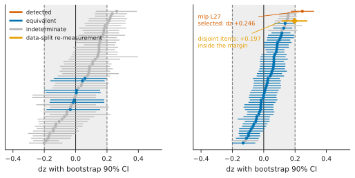
mlp_block__L27 at dz +0.246 — re-measured on disjoint items it returns +0.197, inside the margin, so the reportable arithmetic result is the equivalence, not the detection (§4.4). Intervals are bootstrap only; no power model enters this figure.9Related Work
How This Paper Compares: Everyone Ranks, Nobody Tests
| Method / Paper | Objective / Metric | Includes Significance Test? | Includes Power Analysis? | Corrects Selection Bias? |
|---|---|---|---|---|
| HAWQ (Dong et al.) | Hessian Spectrum / Curvature | ❌ No | ❌ No | ❌ No |
| LSAQ (arXiv:2412.18135) | Jaccard Top-K Token Sets | ❌ No | ❌ No | ❌ No |
| FP4 Diagnosis (Cim et al., 2026) | WikiText-2 Perplexity | ❌ No | ❌ No | ❌ No |
| SliderQuant (ICLR 2026) | Perplexity Sensitivity | ❌ No | ❌ No | ❌ No |
| This Paper | Per-Capability Item NLL & McNemar | ✅ Yes | ✅ Yes | ✅ Yes |
9.1 · The Nearest Neighbor: FP4 Diagnosis Names This Project as Future Work
Cim, Topcu & Kandemir, “Diagnosing FP4 Inference: A Layer-wise and Block-wise Sensitivity Analysis of NVFP4 and MXFP4”, ICLR 2026 Workshop on SciForDL (arXiv:2603.08747). They run Qwen2.5 at 0.5B, 7B and 14B under MXFP4 and NVFP4, scored by WikiText-2 perplexity on “256 calibration samples”. Component sensitivity quantizes “one of all seven projection types (Query, Key, Value, Output, Gate, Up, Down) to FP4 at a time, and keep[s] remaining six of them in FP16 across all layers”; block sensitivity is the inverse.
No statistics of any kind — point estimates and rankings, with no significance test, no noise floor, no multiplicity correction, no power analysis, no repeated run.
Their own conclusion names this project as future work:
“Future work should also evaluate FP4 sensitivity on diverse downstream tasks beyond perplexity on WikiText, such as reasoning, coding, and instruction following benchmarks, to better understand how component level quantization effects translate to task specific performance degradation.”
That is the strongest available evidence the question is open — from the group nearest to it.
mlp_block__L0 improves at one end of the model and mlp_block__L27 at the other.9.2 · What Every Located Method Optimizes, and What None of Them Tests
| method | objective | what it optimizes |
|---|---|---|
| HAWQ (arXiv:1905.03696) | Hessian spectrum / second-order curvature | loss-surface sensitivity |
| LIM | cosine similarity between a layer's input and output | representation change |
| LSAQ (arXiv:2412.18135) | Jaccard similarity over top-k token sets | output-set overlap |
| LRP-QViT (arXiv:2401.11243) | layer-wise relevance propagation | attribution to a target class |
| FP4 Diagnosis (arXiv:2603.08747) | WikiText-2 perplexity | corpus-average likelihood |
Two gaps fall straight out of that table.
- Every objective is a proxy or an aggregate. None measures per-capability task performance per item — and a perplexity ranking cannot be split by capability, because perplexity has already averaged the capabilities together.
- This literature ranks rather than tests. No paper I found reports a significance test, a noise floor, a multiplicity correction, a power analysis or a replication. §4 is what happens when that machinery is imported, and is not restated here.
To be clear about credit: the statistics are textbook and are not claimed as findings. The contribution is their absence from this literature, and what that absence costs.
9.3 · A Prior for the Hypothesis — in a Different Setting
Yin, Xu et al., “LoFiT: Localized Fine-tuning on LLM Representations” (arXiv:2406.01563), §5.3:
“Across all models, task-specific distributions peak in some contiguous sets of layers within the same model rather than being widely spread across layers or concentrated in a single layer. ... head sets for different tasks are only mildly overlapping. These findings demonstrate that there is not a single set of heads best for fine-tuning across all tasks.”
Capability-specific localization is therefore established for fine-tuning. That makes my hypothesis well-motivated rather than speculative — and it makes my inconclusive result more interesting rather than less: a phenomenon that holds under fine-tuning does not clearly reproduce under 3-bit quantization with this instrument. Whether the difference is the intervention, the unit (heads vs. blocks), the selection procedure, or simply my power, is not settled here.
9.4 · Depth Structure: SliderQuant
“SliderQuant: Accurate Post-Training Quantization for LLMs”, ICLR 2026 (arXiv:2603.25284): “shallow/deep layers are usually more sensitive to quantization than intermediate layers”, and among edge layers “the most sensitive one is the first/last layer.”
mlp_block__L27 effect split across four chunks of its intermediate dimension. Two chunks carry 58.3% and 57.2%; one carries 8.0%; one runs the opposite way at −4.9%. One chunk posts a larger standardized effect than the whole block despite carrying 57% of the raw effect — because the chunks that contribute little to the effect still contribute their full share of noise to the block measurement.9.5 · Two Tensions With My Results — Stated, Not Buried
(a) Which components dominate — a genuine conflict. FP4 Diagnosis finds MLP up/down projections dominant, with gate and attention substantially less sensitive. I find attn_block__L0 among the strongest, and structure spanning the depth, including mid-depth attention (attn_block__L12, dz +1.349) (§5). Four differences could account for the conflict, and I can settle none of them from my data:
- Metric — retrieval NLL versus WikiText-2 perplexity. (This paper's own thesis, applied to this paper.)
- Format — §3 finds ordering may not survive a one-bit change.
- Granularity — one block at one layer, versus one projection type across all layers at once.
- Capability.
Running their protocol under my metric on the same model would isolate metric from granularity. Not run; not costed.
(b) Negative improvement — an independent sighting. FP4 Diagnosis reports it once, without investigating:
“notably, for 14B under MXFP4, isolating early blocks can even yield negative improvement.”
Their intervention is the inverse of mine — they restore a block to FP16 and find performance does not improve — but the shape is identical: a component whose relationship to quality runs opposite to the expected direction. I cite it as an independent sighting at a different scale, format and metric. §6 adds that the phenomenon is a class of eight rather than one, that it replicates on disjoint items, decomposes to sub-block granularity, is monotone in perturbation strength, and has one proposed mechanism refuted. That a second group ran into it and moved on is worth saying out loud: it is exactly the shape of a finding that ranking-without-testing produces and then discards.
Conclusion & Key Takeaway for LLM Practitioners
Post-training quantization is not a uniform knob:
- At 4-bit, quantization is nearly free — no damage was detected in either capability, which is a failed rejection rather than a demonstrated equivalence (§3) — but at 3-bit, damage strikes long-context retrieval 3.2× harder than arithmetic reasoning.
- Ranking layers without statistical testing leads to false conclusions. Always use standardized effect sizes (dz), correct for selection bias (the Winner's Curse), and validate on fresh data splits before deciding which layers to protect in mixed-precision deployment!
And read point 2 as the actual deliverable. The primary pre-registered test — whether the two capability maps differ — came back inconclusive (ρ = −0.0014, p ≈ 0.50), so nothing here settles whether retrieval and arithmetic live in different layers. What transfers to your deployment is therefore the method, not a verdict: standardized effect sizes instead of raw-metric noise floors, selection correction instead of naive top-k, and fresh-split validation instead of trusting the number that got a component selected in the first place.
•References
Cited inline in the text; this list is the paper's bibliography. Entries marked “used, not cited in prose” are dependencies a reader needs to reproduce the work.
bitsandbytes is the reference implementation my quantizer is validated against.)AAppendix A · Every Interval, Classified by Selection
All are bootstrap 90% intervals on dz (10,000 resamples), the level my equivalence margin implies.
| interval | quantity | status |
|---|---|---|
| [+0.176, +0.319] | mlp_block__L27 arithmetic dz, seed 2024 | post-selection — the only component of 56 to clear the gate, interval computed on the selecting data |
| [+0.119, +0.274] | same component, seed 2025, disjoint items | valid — pre-specified by the time it was drawn; this is the data-split estimate |
| [−0.0364, −0.0226] | mlp_block__L27 retrieval ΔNLL, seed 2025 | valid — pre-specified, disjoint |
| [+0.166, +0.272] | pooled over both draws | partially contaminated — pools a selected with a non-selected sample |
| per-component equivalence intervals (all 56) | every component, not a subset | valid as a set — only the one reported because it was detected inherits selection |